Applicable version(s):
Latest stable release & Development version
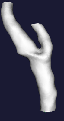
This tutorial demonstrates how to compute centerlines from a surface model of a vascular segment.
Theory overview
Centerlines are powerful descriptors of the shape of vessels. Although the concept of what a centerline is is more or less intuitive, their mathematical definition is not unique. A lot of methods have been proposed in the literature for the computation of centerlines both from angiographic images and 3D models. The algorithm implemented in vmtk deals with the computation of centerlines starting from surface models, and has the advantage that it is well characterized mathematically and quite stable to perturbations on the surface.
For further details please refer to publications and Luca’s PhD thesis.
Briefly, centerlines are determined as weighted shortest paths traced between two extremal points. In order to ensure that the final lines are in fact central, the paths cannot lie anywhere in space, but are bound to run on the Voronoi diagram of the vessel model. There’s a huge literature on Voronoi diagrams, however, as a first approximation, you can consider it as the place where the centers of maximal inscribed spheres are defined. A sphere inscribed in an object is said to be maximal when there’s no other inscribed sphere that contains it. So, for every point belonging to the Voronoi diagram, there’s a sphere centered in that point that is a maximal inscribed sphere (the information relative to the radius is therefore defined everywhere on the Voronoi diagram).
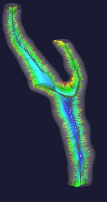
The central figure below shows what the Voronoi diagram (or, more precisely, its internal subset) associated with the shape of a carotid bifurcation looks like. The colors are referred to the radius of maximal inscribed spheres (red: small, blue: large). As you can see, the Voronoi diagram is a non-manifold surface (that is, a surface where different sheets can meet at one edge). One more thing to note is that the Voronoi diagram looks very noisy: small disturbancies on the surface can generate those hair-like structures you see in the diagram (the fact they’re red shows that they are associated with small maximal inscribed spheres). While this is usually a problem for shape analysis, those structures do not affect our centerlines at all, so we just keep them the way they are.
Centerlines are determined as the paths defined on Voronoi diagram sheets that minimize the integral of the radius of maximal inscribed spheres along the path, which is equivalent to finding the shortest paths in the radius metric. They way this is done is by propagating an wave from a source point (one endpoint of the centerline) using the inverse of the radius as the wave speed and recording the wave arrival time on all the points of the Voronoi diagram, and then backtracing the line from a target point (the other endpoint of the centerline) down along the gradient of arrival times. The propagation is described by the Eikonal equation and in the code it is computed using the Fast Marching Method. Clearly, since centerlines are defined on Voronoi diagrams, each point of a centerline is associated with a corresponding maximal inscribed sphere radius.
Using vmtkcenterlines
The script that allows to compute centerlines in vmtk is vmtkcenterlines. It takes in input a surface and spits out centerlines, the Voronoi diagram and its dual, the Delaunay tessellation (or, better, the subset of the Delaunay tessellation internal to the surface).
If you type vmtkcenterlines --help you’ll get quite many options, we’ll now overview of the most important ones. Say you have a model of a vessel in the usual foo.vtp file and you want to compute centerlines out of it. If you write
vmtkcenterlines -ifile foo.vtp -ofile foo_centerlines.vtp
a render window will pop up, asking you to specify points on the surface that will act as source points
Please position the mouse and press space to add source points, 'u' to undo
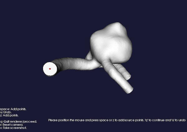
Figure 1: Placing source seeds
When you’re satisfied press q (Note: you really have to click on mesh points to make the selection (a red sphere should appear). If you can’t do it, try to zoom close to the desired point). Now you’ll be prompted:
Please position the mouse and press space to add target points, 'u' to undo
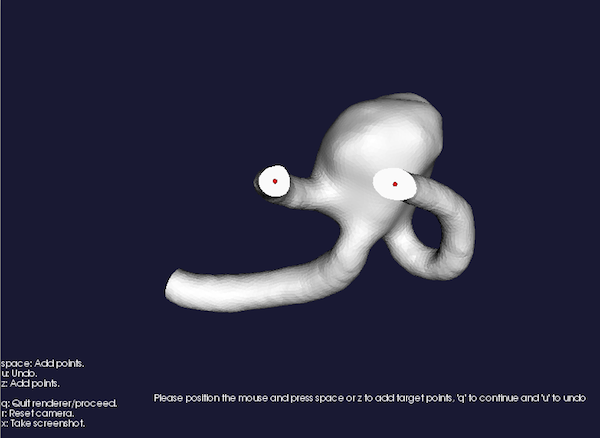
Figure 2: Placing target seeds
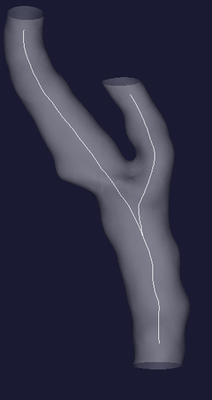
same as above. After you press q the computer will start crunching numbers (mainly those needed to compute the Delaunay tessellation, which is quite an expensive operation). At the end, you’ll have your centerline. Note that on every centerline an array (named by default MaximumInscribedSphereRadius) is defined. You can look at the results this way
vmtksurfacereader -ifile foo.vtp --pipe vmtkcenterlines --pipe vmtkrenderer --pipe vmtksurfaceviewer -opacity 0.25 --pipe vmtksurfaceviewer -i @vmtkcenterlines.o -array MaximumInscribedSphereRadius
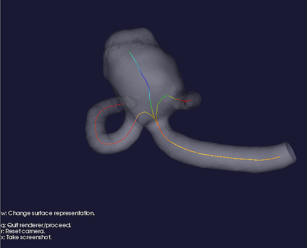
Figure 3: Centerlines visualization.
If you want to take a look at the Voronoi diagram with centerlines defined on it, do the following
vmtksurfacereader -ifile foo.vtp --pipe vmtkcenterlines --pipe vmtkrenderer --pipe vmtksurfaceviewer -opacity 0.25 --pipe vmtksurfaceviewer -i @vmtkcenterlines.voronoidiagram -array MaximumInscribedSphereRadius --pipe vmtksurfaceviewer -i @vmtkcenterlines.o
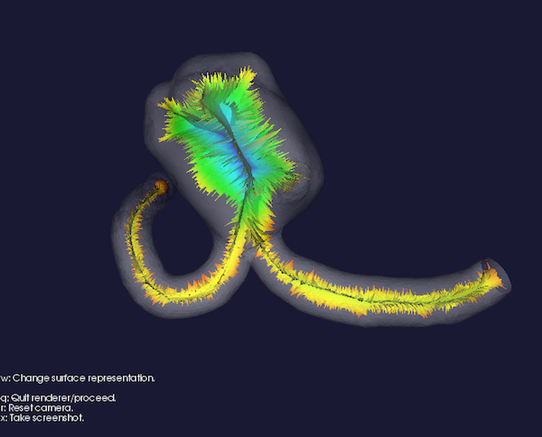
Figure 4: Voronoi diagram
If you inspect the centerlines closely, you’ll notice that they don’t exactly reach seed and target points, but they just go close to them. The reason is that centerlines lie on the Voronoi diagram, and the Voronoi diagram does not touch the surface (for the ones interested, centerlines stop at the poles associated with seed and target points; look here) to find out what poles are). If you want centerlines to end precisely at source and target points, specify the option -endpoints 1: this way the segments from sources and targets to their respective poles are appended to the centerlines.
In the case your model is open-ended, you can also specify seeds and targets as the barycenters of the open profiles of your model. You do this by issuing
vmtkcenterlines -seedselector openprofiles -ifile foo.vtp -ofile foo_centerlines.vtp
The usual render window will pop up, showing the model with all the open profiles identified by a number. After pressing q you’ll see
Please input list of inlet profile ids:
and you’ll have to specify the (space separated) list of ids corresponding to the profiles where you want source points to be defined. You’ll then be prompted
Please input list of outlet profile ids:
and you’ll have to do the same with target points (I named them inlet and outlets instead of source and target… I’ll have to make up my mind at some point!). Anyway, past this point you’ll just have to wait for your centerlines to be computed.
That’s about it for this example. See you next tutorial!