Applicable version(s):
Latest stable release & Development version
This tutorial demonstrates how to generate an image based surface model from a vti image. If you are not sure about how to create or adjust a vti image please refer to the Getting Started section.
Level Sets
There’s a huge amount of literature concerning level sets, so refer to that if you don’t know what they are. For now we’ll just say that level sets are a kind of deformable model in which the deformable surface is not represented by a set of points and triangles, but rather described by a 3D function (basically another image) whose contour at level zero is the surface in question. In practice, the output of a level set segmentation is an image. To extract the surface from the image you have to run the output image through Marching Cubes with level 0. The advantage of using a deformable model (either explicit or level sets) is that the location of the surface will not depend on the level you choose, but instead it will locally conform to the peaks of the gradient modulus of the image levels. In other words, the final surface will be located on the regions corresponding to the steepest change of image intensity across the vessel wall, which is a robust and objective criterion.
In order to use level sets in vmtk you have to use vmtklevelsetsegmentation:
vmtklevelsetsegmentation -ifile image_volume_voi.vti -ofile level_sets.vti
Recall that -ifile and -ofile are ways to access the built-in readers and writers that every script has. The file format is guessed from the filename extension.
First a render window appears displaying the usual image planes.
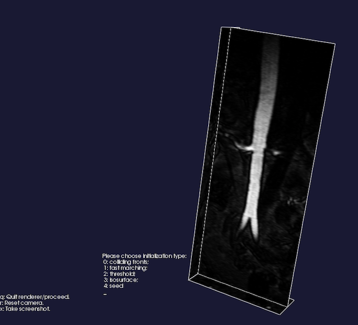
Figure 1: Choosing initialization type
A message will appear:
Please choose initialization type: (0: colliding fronts; 1: fast marching; 2: threshold; 3: isosurface)
This lets you choose the way in which your deformable model is initialized. The goal is to initialize the model as close to the vessel wall as possible.
Colliding Fronts: This initialization type consists of placing two seeds on the image. Two fronts will be propagated from the seeds (one front from each) with their speeds proportional to the image intensity. The region where the two fronts cross,(or collide) is then the initial deformable model. This type of initialization is very effective when it is necessary to initialize the tract of a vessel. For example, by placing a seed at each of the two extremities (thus, two seeds total), the region between the seeds will then be selected. An advantage to this method is that side branches will be ignored.
Fast Marching: This initialization type consists of placing a set of seeds and a set of targets on the image. A front is then propagated from the seeds until the first target is met at which point the region covered by the front is the initial deformable model. This type of initialization is effective when it is necessary to segment round objects such as aneurysms. For example, by simply placing one seed at the center and one target on the wall, the volume will be initialized.
Threshold: With this initialization type, pixels comprised within two specified thresholds will be selected as the initial level sets.
Isosurface: With this initialization type, initial level sets will correspond to an isusurface of the image with sub-pixel precision.
By using level sets it becomes possible to reconstruct a vessel in separate chunks and then merge the results of the different chunks into a single, cohesive, final model i.e. it is not necessary to initialize the whole vessel of interest in one shot. One can proceed, in steps, mixing initialization types, which, can be quite handy. Additionally, it is also possible to save level sets into a file and resume the segmentation later on, adding the results to the first model.
Continuing on with the example:
Enter 0 to initialize with colliding fronts.
A message will then appear:
Please input lower threshold ('n' for none):
Wave propagation can be restricted to a set of intensity levels above a lower threshold and below an upper threshold. This is useful when you don’t have a great SNR in you images. The use of such thresholds is optional, and in general they do not influence the location of the final surface. If you don’t know what the right threshold is, press i to activate the image and probe it. Quit with q when probing is done. Next, enter the value returned by the probe on the terminal. If you don’t want to use any threshold, just enter n (give this a try before using thresholds).
The next message is:
Please input upper threshold ('n' for none):
The above procedure applies here as well.
Next, you’ll be prompted with:
Please place two seeds (click on the image while pressing Ctrl).
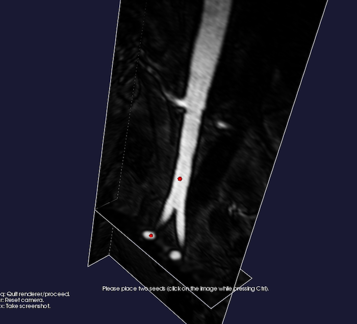
Figure 2: Placing seeds on the image
Interact with the image planes to find the image plane where you want to place your first seed. When satisfied, press the Ctrl key. While keeping it depressed, left-click the image plane on the point you wish to place the seed at. A red sphere will then appear. Repeat this procedure for the second seed as well. Press q when done.
Provided everything went ok, a translucent surface will appear in the render window between the two seeds. This is your initial deformable model. Press q to proceed.
You’ll be asked:
Accept initialization? (y/n):
If you reply n, you’ll be allowed to perform the initialization once again.
The following message will now appear:
 Please input parameters (type return to accept current values, 'q' to quit):
 NumberOfIterations(0) [PropagationScaling(1.0) CurvatureScaling(0.0) AdvectionScaling(0.0)]:
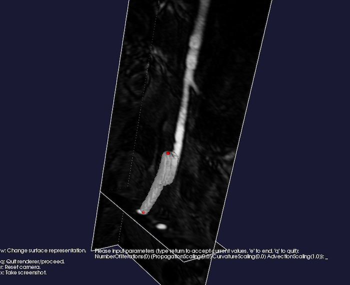
Figure 3: Set parameters to control the deformation of level set.
These parameters control the deformation of your level set.
Number of iterations is the number of deformation steps the model will perform. For numerical reasons, the distance the model will travel will depend on a number of things, among which are voxel size and image gradient modulus intensity.
Propagation scaling is the weight you assign to model inflation.
Curvature scaling is the weight you assign to model surface regularization (this will eventually make the model collapse and vanish if it’s too strong)
Advection scaling is the most important weight. It regulates the attraction of the surface of the image gradient modulus ridges, which is ultimately what you want.
From experience it is recommended that propagation and curvature should be set to 0.0, and advection to 1.0. This is possible if the initialization is sufficiently close to where you want the surface to converge. The number of iterations should be set large enough for the level set not to move anymore (if the region isn’t too big, try with 300). Experiment with the images to see what happens. Keep in mind that setting advection to 1.0 and propagation and curvature to 0.0 will robustly lead you to reproducible results.
Therefore, enter:
300 0 0 1
You can also simply enter
300
as the remaining 0 0 1 are the default.
The level sets will then evolve until the maximum iterations are reached. Progress toward the maximum number of iterations will be displayed as a percentage while processing. At this point, the render window will activate, displaying the final model.
If q is entered instead of 300, the script quits, thus piping the resulting level set to the writer. Don’t do that unless you made an unrecoverable mistake and you’d like to start over again.
To quit the render window press q as usual.
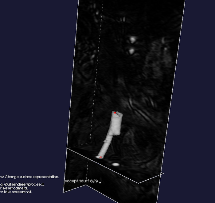
Figure 4: Displaying the final model
You’ll then be asked:
Accept result? (y/n)
- If n, you’ll go back to the level sets parameter question (keeping the same initialization).
-
If y, you’ll go on to the next question:
Merge branch? (y/n)
- If n, this branch will be discarded.
- If y, this branch will be merged with the branches you segmented before.
The render window will show you the merged result.
The next (and last) question will be:
Segment another branch? (y/n)
- If y, you’ll be sent to the initialization stage.
- If n, the script will quit and merged result will be sent to the writer.
At this point you have a file named level_sets.vti which contains an image (which you can display for examination using vmtkimageviewer). The zero level of this image is the surface you generated. Therefore, now extract a polygonal surface from it:
vmtkmarchingcubes -ifile level_sets.vti -ofile model.vtp
If you wanted to do everything in one shot you could have done:
vmtklevelsetsegmentation -ifile image_volume_voi.vti --pipe vmtkmarchingcubes -i @.o -ofile model.vtp
Two points to be made:
- It is necessary to specify the piping from level sets to Marching Cubes explicitly (with -i @.o) because the name of the output argument from vmtklevelsetsegmentation is LevelSets and not Image as vmtkmarchingcubes expects by default.
-
It is suggested that an image file of level sets are kept. This allows you to add branches later on by simply doing:
vmtklevelsetsegmentation -ifile image_volume_voi.vti -levelsetsfile level_sets.vti -ofile level_sets2.vti
That’s it.
Don’t forget to explore the options that the scripts offer. If you’re in doubt, mail us a question, either personally or on the mailing list (see the vmtk homepage for details).