Applicable version(s):
Latest stable release & Development version
by Marina Piccinelli, Math CS Department, Emory University, Atlanta, US
This tutorial demonstrates how to map the surface of a population of vessels onto the same parametric space and enable statistical analyses of surface-based quantities.
Overview
The theory behind this tutorial can be found in details in the following publication:
- Antiga L, Steinman DA. Robust and objective decomposition and mapping of bifurcating vessels. IEEE Transactions on Medical Imaging, 23(6), 2004.
Briefly, each segment of a vascular network is topologically equivalent to a cylinder and can consequently be mapped onto a rectangular parametric space that allows both easier investigations and comparisons between different models and datasets. The parameterization is performed longitudinally by means of the curvilinear abscissa computed over the model centerlines and circumferentially, by the angular position of each point on the surface mesh with respect to the centerlines.
Pre-requisites
In addition to ad hoc vmtk scripts for metric calculation (vmtkbranchmetrics), mapping (vmtkbranchmapping) and patching (vmtkbranchpatching), this tutorial relies on concepts and operations presented in previous sections, such as centerlines extraction, their geometric analysis, bifurcations identification and branch splitting.
An example: WSS and OSI along a branching vascular district
A common application is mapping and patching of fluid dynamics variables, such as wall shear stress (WSS) or oscillatory shear index (OSI), obtained on the surface mesh typically by means of a CFD simulation.
Let’s assume we have the mesh surface depicted in Figure 1: it represents the aorta of a mouse with its main branches (from top to bottom: celiac, mesenteric and right renal arteries) for which the WSS and OSI were computed.
The surface model was provided by T. Passerini, Math&CS Department, Emory University, Atlanta, US.
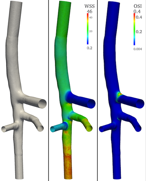
Figure 1. 3D model of a mouse aorta and its main branches with associated WSS and OSI attributes
We will refer to the mesh surface as aorta.vtp; we also assume, even if it is not mandatory, that dimensions are in mm.
Here are the steps you may want to follow to patch and flatten the surface:
Centerlines extraction and branch splitting
We extract the centerlines from the model, compute their attributes, i.e. the curvilinear abscissa and the parallel transport normals system - both attributes are crucial for the surface parameterization - and split them (Figure 2-left).
vmtkcenterlines -ifile aorta.vtp --pipe vmtkcenterlineattributes --pipe vmtkbranchextractor -ofile aorta_cl.vtp
Bifurcation reference systems
We compute the bifurcation reference systems along the centerline network just computed
vmtkbifurcationreferencesystems -ifile aorta_cl.vtp -radiusarray MaximumInscribedSphereRadius -blankingarray Blanking -groupidsarray GroupIds -ofile aorta_cl_rs.vtp
Surface splitting
We subdivide the surface in its constituent branches: in this way the mapping and patching will be performed on each singular branch (Figure 2-right).
vmtkbranchclipper -ifile aorta.vtp -centerlinesfile aorta_cl.vtp -groupidsarray GroupIds -radiusarray MaximumInscribedSphereRadius -blankingarray Blanking -ofile aorta_clipped.vtp
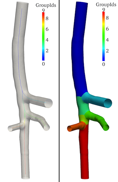
Figure 2. Split centerlines (left) and surface (right): GroupIds array shown.
Longitudinal and circumferential metrics
By means of the vmtkbranchmetrics script two additional arrays are created on each branch of the split surface whose default names are AbscissaMetric and AngularMetric: the first is computed from the curvilinear abscissa defined on the centerlines, while the second represents the periodic circumferential coordinate of mesh points around the centerlines and spans the interval (-π, +π). In Figure 3 iso-contours over the two arrays are also shown.
vmtkbranchmetrics -ifile aorta_clipped.vtp -centerlinesfile aorta_cl.vtp -abscissasarray Abscissas -normalsarray ParallelTransportNormals -groupidsarray GroupIds -centerlineidsarray CenterlineIds -tractidsarray TractIds -blankingarray Blanking -radiusarray MaximumInscribedSphereRadius -ofile aorta_clipped_metrics.vtp
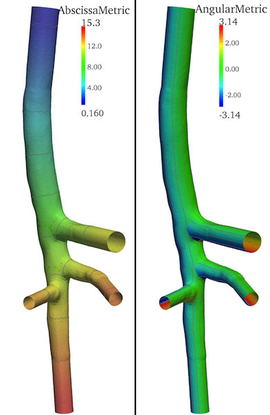
Figure 3. Longitudinal (left) and circumferential metrics created over the surface model by vmtkbranchmetrics script; iso-contours over the two fields are shown.
Metrics mapping to branches
By construction of a harmonic function (Figure 4-left) over each vascular segment, vmtkbranchmapping maps and stretches the longitudinal metric to correctly account for the presence of insertion regions at bifurcations; the additional StretchedMapping array is added to the surface (Figure 4-middle).
Try the command
vmtkbranchmapping --help
to verify all the information needed by the script: results from vmtkbranchmetrics, centerline attributes and arrays, information about the bifurcation geometry.
vmtkbranchmapping -ifile aorta_clipped_metrics.vtp -centerlinesfile aorta_cl.vtp -referencesystemsfile aorta_cl_rs.vtp -normalsarray ParallelTransportNormals -abscissasarray Abscissas -groupidsarray GroupIds -centerlineidsarray CenterlineIds -tractidsarray TractIds -referencesystemsnormalarray Normal -radiusarray MaximumInscribedSphereRadius -blankingarray Blanking -angularmetricarray AngularMetric -abscissametricarray AbscissaMetric -ofile aorta_clipped_mapping.vtp
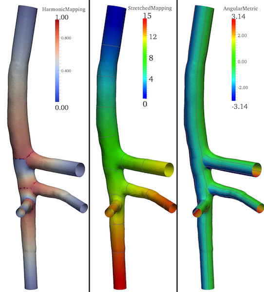
Figure 4. Harmonic funtion built over each branch (left); stretched longitudinal metric (middle) and angular metric (right).
Patching of surface mesh and attributes
All the ingredients are now in place to perform the real patching of the surface, that is to “cut” a set of contiguous rectangular regions on the mesh that follow iso-contours in the StretchedMapping and AngularMetric arrays; all the quantities of interest (WSS and OSI in this case) are averaged over these areas.
Try the help command the see the information needed
vmtkbranchpatching --help
By means of the options -longitudinalpatchsize and -circularpatches we impose the dimensions of the patches, in terms of “height” (in mm) of the patch along the longitudinal direction and number of angular cut over the interval (-π, +π) respectively; the result of this discretization can be seen visualizing the Slab and Sector arrays created by the script or the mesh new surface discretization (Figure 5). You’ll probably have to play with these values to find out the discretization that best fits your needs; we here cut every 0.5 mm and subdivide the interval (-π, +π) in 12 sectors.
vmtkbranchpatching -ifile aorta_clipped_mapping.vtp -groupidsarray GroupIds -longitudinalmappingarray StretchedMapping -circularmappingarray AngularMetric -longitudinalpatchsize 0.5 -circularpatches 12 -ofile aorta_clipped_patching.vtp
Figure 5. New mesh tesselation created by vmtkbranchpatching by cutting the surface longitudinally and circumferentially.
Figure 6 shows the patching of the data attributes over the surface.
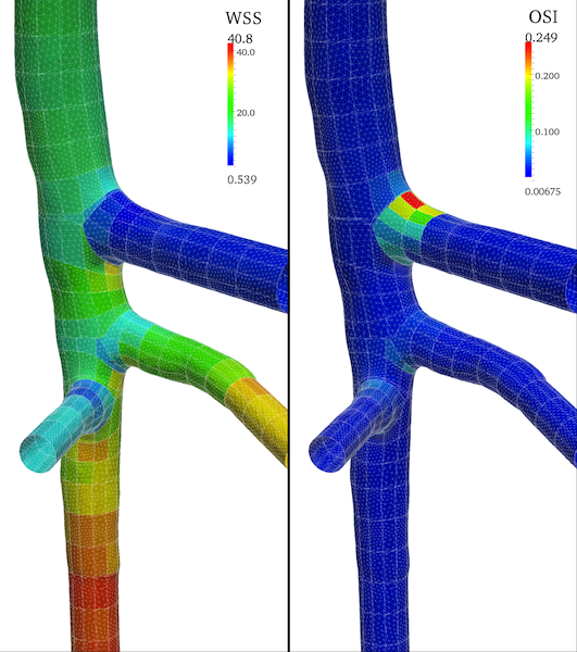
Figure 6. Surface model with patched WSS and OSI attributes; the mesh tesselation is also displayed.
By adding the following option to the previous patching command the patched data will be flattened and exported as a .vti image or a .png (.jpg, .tiff, etc). Figure 7 shows the patched 3D surface (WSS is visualized) and the flattened WSS (middle) and OSI (right) images. By default in the final .vti (or .png) images the flattened patched dataset of each branch are vertically juxtaposed.
-patcheddatafile aorta_clipped_patching.vti or -patcheddatafile aorta_clipped_patching.png
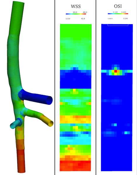
Figure 7. Left: 3D patched dataset (WSS displayed) for the complete model; middle and rigth: flattened images of patched WSS and OSI for the whole vascular network by vertical juxtaposition of each branch portion.
Extraction of one branch
One possible way to extract the patched 3D surface and the flattened image for only one of the vascular branches is to use vmtkbranchclipper to clip the segment of interest before performing the patching. For example to extract the branch with group id 5
vmtkbranchclipper -ifile aorta_clipped_mapping.vtp -groupids 5 -groupidsarray GroupIds -blankingarray Blanking -centerlinesfile aorta_cl.vtp -radiusarray MaximumInscribedSphereRadius --pipe vmtkbranchpatching -circularpatches 12 -longitudinalpatchsize 0.5 -longitudinalmappingarray StretchedMapping -circularmappingarray AngularMetric -ofile aorta_clipped patching_id5.vtp -patcheddatafile aorta_clipped_patching_id5.vti
Figure 8 shows the results.
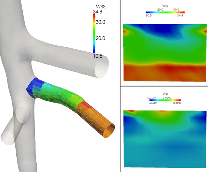
Figure 8. 3D patched surface and flattened images for the branch #5.
By means of the flattened images, comparisons or correlations between different models or different datasets are readily computable.